Unfiltered: Automatic Identification and Inversion of Social Media Photography Filters

Mert Dumenci, Cem Gokmen, Chunlok Lo, Joel Ye
CS4476 Term Project, Fall 2018
Georgia Tech

Abstract

Given the prevalence of photo editing and filtering on popular social media platforms such as Snapchat and Instagram, it is becoming more and more difficult for users to identify how the content that they consume everyday have been modified from their original form. Since filtering has become so common, the goal of this project is to give users a means to identify how photos on these platforms are edited and to present a plausible reconstruction of source content.

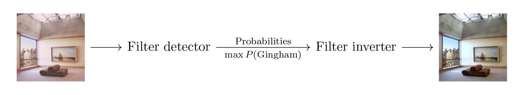
We propose an end-to-end system that will take an image from the user, identify probabilities for which common image filters were applied to the image, and apply the most likely filter inverse. We present both the filter probabilities and the inverted image to the user. For filter identification, we utilize a convolutional neural network to determine a probability vector for possibly applied filters. For filter inversion, we model an inverse convolution kernel for each pre-defined filter using a neural network and apply the convolution over the image to obtain the inverted image.

Using our approach with a convolutonal neural network, we can identify a filter applied to an image (from our predefined set of six Instagram filters) while distinguishing it from natural (unfiltered) images with an accuracy of $95.5\%$.

Let $E(I, I')$ be the average per-pixel mean of the sum absolute differences in intensity across all color channels of images $I$ and $I'$ (Equation 1). For inverting images given a known filter, we are able to obtain a pseudo-inverse of the image with an average error $E$ of $1.0\%$.

Our end-to-end system detected and inverted filters with an average error $E$ of $1.7\%$ between our output image and the original unfiltered version. In comparison, the baseline error $E$ between filtered and unfiltered images was found to be $8.4\%$ while our previous approach using color histograms achieved $5.5\%$.

Teaser Image

Introduction

Filtered photos have become ubiquitous on social media platforms such as Snapchat, Instagram, Flickr, and more. To the casual viewer, filters can be hard to detect. Their intentional subtlety makes it hard to distinguish between filtered and unfiltered images on social media. This can lead to distorted perceptions of natural images, skewing expectations about natural appearances. We hope this project will help bring more transparency into how images are often edited by identifying whether a common image filter has been applied to an image, and expose users to the natural state of these images. We believe that transparency in the image editing process is important in raising awareness about deliberate modifications to perceptions of reality, and hope to allow viewers to enjoy edited content while being aware of their modifications.

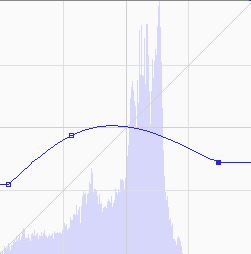
Not to be confused with filters in the computer vision setting, which are generally used in image preprocessing, filters in the social media setting describe a predefined set of modifications to an image that attempts enhance its perceptual appeal. Most commonly, these filters come in the form of color balance adjustments and can be represented as tweaks to the color curves of an RGB image. A color curve $f: [0, 255] \to [0, 255]$ is a continuous function that remaps the intensities in each color channel. Modification to the color curve allows the user to non-uniformly boost or decrease color intensities at varying ranges to create various effects such as increasing contrast or creating color shifts (figure below demonstrates a boost of blues in shadows while decreasing blues in highlights.)

Some filters also include additional effects such as blurring/sharpening using convolution kernels, the addition of borders, and the application of vignette darkening at the edges.

Before filtering	After filtering
Original Image	Filtered Image
Color Curve Before Filtering	Color Curve After Filtering

For the purposes of this project, we limit our scope and define a filter as a pair $(f, g)$ where $f: \mathbb{R}^3 \rightarrow \mathbb{R}^3$ is a function that maps every individual color (consisting of 3 channels each with a real value in the $[0, 1]$ range) to some color in the same range, and $g \in \mathbb{R}^{3 \times 3}$ is a convolution kernel that can be used for blurring and sharpening among other effects. We assume that a filter is applied first by passing each pixel of an image through $f$, and then convolving the image with $g$, extending the edges by repeating the last row and column of pixels as to preserve the shape of the image.

While many commercial filters may also contain additional effects such as borders and vignettes, filters are mostly characterized by how they shift the color curves globally and their blur/sharpen/emboss effects. Therefore, for the scope of this project, we choose filters which do not have these additional effects.

Though our work relates to many other fields of computer vision, such as image denoising and brightening images, not much work directly focuses on end to end filter identification and inversion. One publication that we found for identification depends heavily on prior knowledge of the camera demosaicing algorithm which is not always readily available^[1].

In many of these settings, such as image denoising or brightening, the modifications applied to the image (noise, etc.) are either consistent across the dataset or are known a priori. Our task is different from this previous work as our filter functions are unknown, but we have examples of unfiltered and filtered images. Therefore, we decompose this task of filter inversion into two separate tasks: filter identification given an input image, and filter inversion given a known filter. Filter identification for an image is a classification task while filter inversion is a regression task estimating the filter inverses.

However, the task of filter identification has a similar formulation to the problem of source camera identification, where one attempts to identify the source camera of an image from a list of possible cameras. There have been several pieces of literature, especially in the field of digital forensics, that attempts to model sensor noise patterns explicitly and build correlations between noise patterns and camera source^[1:1] but have failed to achieve high accuracy. However, several recent works have applied convolutional neural networks to the problem and achieved notable results^{[2] [3] [4]}. Because the problem formulation between source camera identification and filter identification is similar, we take inspiration from the approach of these recent papers and apply it to the context of filter identification. For filter inversion, we formalize our definition of filters and use a neural network to model the kernel of an inverse filter convolution function.

Approach

Our approach splits the end-to-end task of filter inversion into two steps:

• Generate a probability vector for possible filters applied to a given image. (Filter identification)
• With the image and the probability vector as inputs, apply a learned inverse filter onto the image to recover the unfiltered image. (Filter inversion)

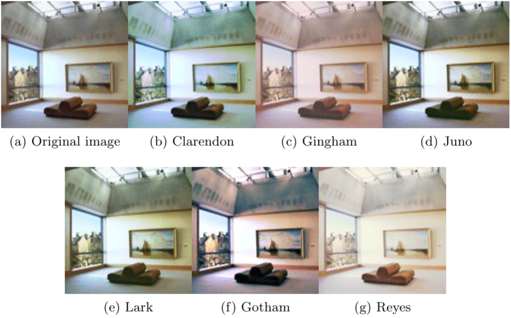
While there are infinitely many filters possible, popular social media platforms have a few pre-selected filters that are widely used. Therefore, we constrain the scope of our filter inversion by assuming input images were filtered at most once by a filter from a known set. To accurately model a real-world application, our list comprises of the following six popular Instagram filters:

Given the scant amount of existing literature on the problem of filter identification, there are no established processes for filtering large numbers of images using commercial filters. We were prompted to create our own image filtering pipeline. Since Instagram filters are not available outside of their platform, we imitated these filters by manually specifying color curve adjustments for each filter. We referenced channel adjustment code from an online article ^[5], which uses numpy functions, specifically linspace and interp, to modify the color curves of each specific channel. We obtained curve parameters for each filter from an online reference^[6] and passed them onto the channel adjustment code to create an imitation of commercial filters. We then run each imitation filter over our library of unfiltered images to create our dataset.

Filter Identification

Our approach to filter identification takes in an input image and outputs a probability vector for the possible filters applied to the input image. We utilize a neural network model to generate this probability vector from the input image.

As convolutional neural network architecture was able to obtain good results in the problem of source camera identification, we follow the architecture detailed in the paper by D. Freire-Obregon^[2:1] and apply their technique to this problem space.

We utilize Keras^[7] to create a convolutional neural network that takes in $32 \times 32 \times 3$ images, pass them through two convolutional layers, one max pool layer, and two fully connected layers. We then pass this output through a softmax layer which provides us a probability vector of filter guesses. We use categorical cross-entropy loss function and the Adam optimizer ^[8] to train our neural network model.

Additionally, the network contains an activation layer after every single layer with the exception of the output softmax layer. We compared the use of ReLU and leaky ReLU^[9] activation functions in our network. We found that leaky ReLU generally provided quicker training and higher accuracies hence our selection.

While many approaches described in camera source identification literature utilize regularization and dropout layers to reduce overfitting in the training process, we have found little evidence of overfitting in our network due to our large number of training examples (over 900k images). Therefore, we did not use any regularization and dropout layers instead saved models after each epoch and took the model at which validation accuracy is maximized and thus before overfitting occurs.

Network Architecture Diagram^[2:2]

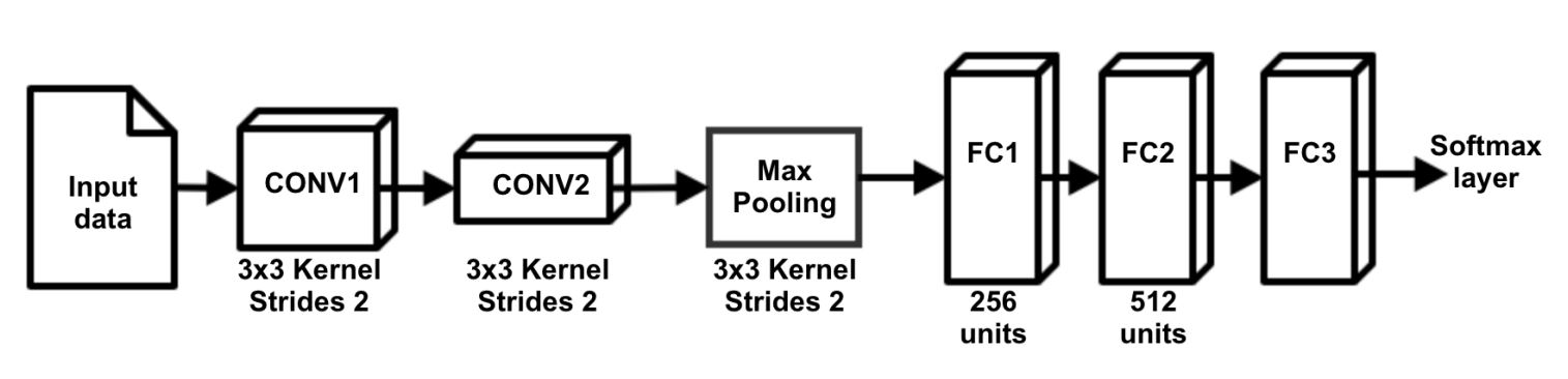
Our architecture is derived from the Obregon paper^[2:3] with leaky ReLU activation layers after all non-output layers. We use 32 kernels for each convolutional layer which performed the best in our experiments.

Because the architecture presented in the paper only processes $32 \times 32 \times 3$ images while our dataset and input consisted of larger images, we developed our own routines to divide our input image into separate $32 \times 32 \times 3$ patches. During prediction time, a majority voting scheme is used to form the final prediction using the prediction results from each patch. We take the a prediction vote from every subpatch of the image and take the mode of that data as the final prediction.

This makes our architecture adaptable to various image sizes and has experimentally been shown to further increase prediction accuracy in comparison to classifying individual $32 \times 32 \times 3$ images.

To avoid memorization and incorrect evaluation results, we ensure that all filtered version of an image from our dataset belongs to the same training, testing, or validation set. In this setup, the identification network has never seen the images presented to it in testing and validation in any form, which results in a better approximation of a practical use for the model.

Filter Inversion

For the inversion of filters, our formalization of a filter is critical. We assume the definition of a filter as a pair $(f, g)$ of a function $f$ that maps colors to colors, and a convolution kernel $g$.

With this assumption, we design a set neural networks to approximate the behavior of an inverse filter. The specification of the neural network for one filter $(f, g)$ is such that given a $3 \times 3$ region of pixels, it should be able to learn and undo the convolution $g$ centered at the middle of the square, then learn and apply the inverse of the function $f$, finally outputting the unfiltered color of the middle pixel of the patch.

We set up a neural network model with an input of $3 \times 3 \times 3$ values to represent the RGB colors of the $3 \times 3$ patch, an output of $3$ values to represent the RGB colors of the center pixel. The topology consists of two hidden layers with $100$ neurons each, to account for potential non-linearities of $f$. We note that since $(f, g)$ are specific to each filter, we will need to train a separate copy of this model for each of our supported filters.

Finally, to apply filter inversion to a given image known to be the result of a particular filter $f$, we iterate through the image using a $3 \times 3$ sliding window, and for each step of the iteration we feed the window into the pre-trained inversion model corresponding to $f$. The model outputs the predicted unfiltered color of the pixel at the center of the image, which we store in a copy of the image. Repeating this operation over patches centered at each pixel on the image, we reach the predicted unfiltered image.

Note that due to the fact that our model is based on filter functions that we define and implement, it was also possible to attempt to invert all of our filters deterministically that aimed to undo each step of the filter. However, we do not know the exact functions behind the real filters used on Instagram et al. Such a method, then, would not be applicable on images filtered using filters whose source code we cannot access, such as images on social media. As a direct result of our learning method, given a sufficiently large dataset of filtered images (alongside their unfiltered counterparts), we can learn to invert any filter that our definition of a filter can represent.

Complete Model

We evaluate our complete model by tying together the detector and the inverter. Given an input image, we run the detector to find the most likely applied filter. We get our output unfiltered image by running the corresponding inverter.

End-to-End CNN

Taking inspiration from encode-decoder networks^[10], we also explore building a single network that bypasses discrete steps of classification and neural networks, and instead create a single convolutional network that aims to invert images from the input. The motivation is to allow the identification and inversion of more nuanced filter combinations, rather than forcing an image fit to a single filter’s characteristics. This would provide a plausible generalization of inversion even for unknown filters. We utilized the same architecture as our filter identification step but removed the softmax layer and instead appended an upsampling layer and $3 \times 3$ convolutional layer with 3 kernels.

Experiments/Results

We perform our experiments using 9000 $128 \times 128 \times 3$ images from 10 different categories from the MiniPlaces dataset^[11] passed through 6 different filters^[12] to create a total dataset of 63000 images (including the original images.) We split these images into 89.55% training, 0.45% validation and 10% testing sets with assurance that the sets are closed under filtering. Therefore, our training set consists of 56420 images, our validation set of 280 images, and our testing set of 6300 images.

$$\text{9000 images} \times \text{6 filters} + \text{9000 original images} = \text{63000 training images}$$

$$\text{63000 images} \times 0.8955 \approx 56420$$

$$\text{63000 images} \times 0.45\approx 280$$

$$\text{63000 images} \times 0.1 = 6300$$

Filter Identification

For filter identification, because each image in the dataset is $128 \times 128 \times 3$, we further subdivide each image into 16 non-overlapping $32 \times 32 \times 3$ images for training, leading to a total of $902720$ training images and $4480$ validation images. Each image also has an associated 7-dimensional one-hot output vector that indicates the ground truth for which filter has been applied to the image.

As described in Approach, we adopted the model in the Obregon paper ^[2:4] and found that slight tweaks in the model hyperparameters was sufficient to provide strong results. We test greater modifications to the architecture, such as adding additional convolution layers and tweaking number of neurons in the fully connected layers. We found that decreasing model complexity is generally correlated with decreasing accuracy, and increasing complexity did not strongly correlate with increasing accuracy. One specific hyperparameter we tuned was the negative slope coefficient on the leaky ReLU layers. We found a sweet spot of $0.3$ which allowed fast convergence and robustness to variation of other hyperparameters.

We trained in rounds of $5$ epochs with various batch sizes until validation accuracy started to decrease due to overfitting. Specifically, our results were obtained by training the model with a total of 3 rounds of 5 epochs with batch sizes of $256$, $1024$, and $4096$ on an NVIDIA GTX970M GPU using Keras^[7:1].

To prevent overfitting, we evaluated how many epochs to train using overall accuracy on the validation set. Specifically, we trained until validation accuracy started to decrease and took the model at which validation accuracy is the highest.

For final model evaluation, we evaluated the overall accuracy, precision, recall, and F1-score for each filter category while treating each $32 \times 32 \times 3$ patch in the testing set as an independent image. We also evaluated our model using the same metrics on the testing set by applying the previously described majority voting scheme .

We then compared the CNN approach to the results of our previous approach, where we extracted RGB color histograms as features to an image which were fed into a feed-forward neural network model for classification.

• Baseline accuracy with random decision: $0.143$
• Average accuracy from color histogram features fed into a neural network model: $0.783$
• Average accuracy from color histogram features and scene label fed into a neural network model: $0.802$
• Average accuracy of our convolutional neural network model: $0.955$

Individual Image Patch Classification

$\mu_{accuracy} = 0.839$

	Identity	Clarendon	Gingham	Juno	Lark	Gotham	Reyes
Precision	0.796	0.858	0.918	0.727	0.762	0.892	0.924
Recall	0.855	0.816	0.984	0.774	0.692	0.923	0.827
F1-Score	0.824	0.836	0.950	0.749	0.725	0.907	0.873

Filter Classification using Majority Voting Scheme

$\mu_{accuracy} = 0.955$

	Identity	Clarendon	Gingham	Juno	Lark	Gotham	Reyes
Precision	0.967	0.992	0.974	0.844	0.948	0.979	0.993
Recall	0.977	0.966	1.00	0.952	0.813	0.997	0.980
F1-Score	0.972	0.979	0.987	0.895	0.876	0.988	0.987

Surprisingly, our convolutional neural network achieved dramatically improved performance over our histogram approach. We say surprising, because convolutions focus information on local spatial structures. One hypothesis for this result is that the network is able to learn kernels such that each individual kernel activated in certain patterns in response to the different color curves of the image.

Another surprising fact is that we are able to achieve considerable performance even when subdividing images into $32\times 32\times 3$ images. This indicates that filters applied to these images create global image features regardless of the image content. Further, the convolutional network was able to capture the expected characteristics of images that have been filtered with a particular filter. More impressively, the detection is accurate even for some filters that are hard to distinguish by human classification.

While the individual image filter performance boasted an improved accuracy performance of $0.84$, the results are even better when we account for image subdivision and use majority voting to determine the final prediction. This is because multiple prediction results allow us to be more tolerable of individual classification errors, which may be raised because of the globality characteristic of filters breaking. The subdivision the image into 16 subpatches was enough to allow the correct filter to gain majority vote, regardless of noise in individual patches.

Just as in our histogram approach, the probability that a filtered image might be confused with another filter depends on the similarity of the filtered image to other images. This is especially apparent between Lark and Juno.

Note the interesting asymmetry in the relationship of these misclassification results. For example a significant amount of Lark images have been confused with Juno but not the other way around. This is perhaps due to the effect of filters on different images. Certain filters might have similar effects to other filters only with a certain distribution of colors in the original image. So while the filters effects’ are generally distinct, results might be confusing on specific images.

Filter Inversion

An important task is to train the inversion model with sufficient data to allow it to generalize. To train the model for a specific filter, we generate a $3 \times 3$ RGB image ($3 \times 3 \times 3 = 27$ integers in the range $[0, 255]$) uniformly at random, and apply the filter to this small image. We store the filtered $3 \times 3$ image as an input $x$ and the color of the center pixel of the unfiltered patch as an output $y$. Every such $(x, y)$ forms one sample, and we train our neural network on 1 million such samples until validation score plateaus.

To assess filter inversion performance, we filtered the test images with all of our filters, Reyes, Lark, Juno, Gingham and Gotham, and inverted them with the respective inversion models.

Note that we assume correct knowledge of the filter in this section, and $E_{pp}$ is mean per-pixel absolute error.

Filter	Filtered $E_{pp}$	Inverted $E_{pp}$	Percent undoing of filter
Reyes	$0.20005$	$0.00669$	$96.655\%$
Lark	$0.03894$	$0.00945$	$75.726\%$
Juno	$0.04440$	$0.00742$	$83.288\%$
Gingham	$0.12112$	$0.00403$	$96.670\%$
Gotham	$0.05742$	$0.03005$	$47.673\%$
Clarendon	$0.038308$	$0.00500$	$86.947\%$

Overall, our inversion model has successfully reduced the mean per-pixel color difference of $0.08337$ (in a scale of $[0, 1]$) between original and filtered images to a mean per-pixel color difference $0.01044$ between the original and unfiltered images.

As a result, we claim our model can reverse $81.159\%$ of the mean per-pixel change caused by an average filter.

Complete Model

As both detection and inversion have reliable performance, it’s worth quantifying the performance of the complete system. On average, per pixel error is $1.6\%$, whereas baseline error between the original image and a filtered image is $8.3\%$. This means our system undoes the filter by reducing the pixel offset from the original image by $81\%$ numerically. This result is potentially even better perceptually. This is demonstrated in the qualitative results.

End-To-End CNN

Our end-to-end network failed to perform as well as inversion through our manually discretized steps. The baseline mean absolute per pixel error through our testing set was $8.34 \%$ per channel and our network was able to achieve a mean absolute per pixel error of only $6.67\%$ per channel. Typical encoder-decoder models are highly complex with many layers and neurons to capture scene information, which then are used to transform the data back into an image. This makes it highly probable that the network we tested was too shallow and simple to capture the information needed to recreate the inverted image.

Qualitative Results

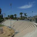
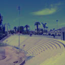
Success cases (Proper Detection)

Filter	Original Image	Filtered Image	Unfiltered Image
Reyes
Clarendon
Juno
Gingham
Gotham
Lark

Failure cases (Predicted filter in parentheses)

Filter (Predicted)	Original Image	Filtered Image	Unfiltered Image
Lark (Juno)
Clarendon (Gotham)
Juno (Lark)
Gotham (Gotham)
Reyes (Gotham)
Gingham (Reyes)

Overall results are almost always perceptually passable. No section is dedicated for qualitative results of inversion, as the complete model’s performance in the success cases are arguably imperceptible from the original images. Occassionally, confused filters led to unnatural coloration (inversion of the wrong filter).

We explain the relative lack of extreme failure cases by observing that our system generally confuses like-filters together. Since these filters have similar inverses, the results are not extreme diversions from the original image. Other mistakes can be further explained by the original images having “unnatural” color distributions, such as scenes in very low-light. Filtered versions of such images might vary significantly from expected images for the same filter. Thus in these failure cases, our system applies the wrong inverse but outputs a more “natural” or normalized photo that has typical color distributions.

Conclusion and Future Work

For filter identification, our approach utilized a convolutional neural network architecture inspired from work in camera source identification^[2:5] and were able to achieve an average accuracy of $95.5\%$ across a set of 6 filters, each with a different effect on the color curves of an image.

For filter inversion, our trained neural network kernel models can invert known filters with an average error $E$ (Equation 1) of $1\%$ across our 6 filters, compared to the baseline error of $8.4 \%$.

With these approaches combined, our complete model achieves an error $E$ (Equation 1) of $1.6\%$, whereas in comparison, the baseline error is $8.4\%$ between filtered and unfiltered images. In other words, our complete model on average is able to reverse $1 - \frac{1.6\%}{8.4\%} = 81\%$ of the effect of a filter on an image.

We initially planned to continue exploring more structured approaches extracting expert features after we extracted color histograms and scene context as image features in a decision model. However, the recent successes of convolutional neural networks in camera source identification^{[2:6] [3:1] [4:1]} guided us to further explore CNN approaches. In the end, our approach using CNNs in filter identification outperformed our previous models by over $17.5\%$ accuracy.

Our end-to-end encoder-decoder model only achieved a result of a mean absolute per pixel error of only $6.67\%$ per channel. This not only failed to beat our two-step inversion model error of $1.7 \%$, but also failed to have a significant improvement on the baseline error of $8.4\%$.

Right now, this application is usable as a Python library. One avenue of future work can be the implementation of a wrapper around popular social media websites and apps that applies our solution on each image before displaying the image to the user. Our models, completely developed using popular APIs such as Tensorflow, are fully usable as a browser plugin, which makes this a natural next step. Such a product would make the process of image unfiltering effortless and would allow users to view unfiltered / unmodified content without leaving their social media feeds.

Ultimately, this project has been a proof of concept. To be even more applicable to real world usage, it should support any combination of filters at various intensities and advanced effects such as vignetting. However, inversion such effects are expected to be harder and we did not tackle such problem for this project.

One possible step towards supporting the above features would be to create a more flexible classifier and inverter. We would create models that can describe the filtering done to an image in a high dimensional feature space and models that can invert an image based on the obtained filter embedding. For example, we can take the output of the last hidden layer in our identification network and create a new inversion model to accept a filter feature vector alongside the image as input. Such model will be more capable of handling a greater variety of filters applied at different intensities and be able to revert a greater variety of edited images. Our success in the more constrained problem with a fix set of filters motivates consideration in designing and testing model architectures that can solve the more general problem.

The increased complexity required for this kind of system naturally matches the complexity of the supported filtering processes. There remain many avenues for progress in the problem of identifying and inverting edited images.

---

1. J. Lukas, J. Fridrich, and M. Goljan, “Digital camera identification from sensor pattern noise.”, IEEE Transactions on Information Forensics and Security, 2006. ↩︎ ↩︎

2. D. Freire-Obregon, F. Narducci, S. Barra, and M. Castrillon-Santana. “Deep learning for source camera identification on mobile devices”, arXiv, 2017. ↩︎ ↩︎ ↩︎ ↩︎ ↩︎ ↩︎ ↩︎

3. N. Huang, J. He, N. Zhu, X. Xuan, G. Liu, and C. Chang. “Identification of the source camera of images based on convolutional neural network”, Digital Investigation, 2018. ↩︎ ↩︎

4. A. Kuzin, A. Fattakhov, I. Kibardin, V. Iglovikov, and R. Dautov. “Camera Model Identification Using Convolutional Neural Networks”, arXiv, 2018. ↩︎ ↩︎

5. M. Pratusevich, “Instagram Filters in 15 Lines of Python”, Practice Python, 2016. Retrieved from URL. ↩︎

6. GraphixTV, “Instagram Filter Effects Tutorials”, YouTube, 2017. Retrieved from URL ↩︎ ↩︎

7. F. Chollet and others, “Keras”, GitHub, 2015. ↩︎ ↩︎

8. D. P. Kingma and J. Ba, “Adam: A Method for Stochastic Optimization”, 3rd International Conference for Learning Representations, San Diego, 2015. ↩︎

9. Bing Xu and Naiyan Wang and Tianqi Chen and Mu Li, " Empirical Evaluation of Rectified Activations in Convolutional Network", arXiv, 2015. ↩︎

10. Vijay Badrinarayanan, Alex Kendall, Roberto Cipolla, Senior Member, IEEE, “SegNet: A Deep Convolutional Encoder-Decoder Architecture for Image Segmentation”, arXiv, 2017. ↩︎

11. B. Zhou, A. Lapedriza, A. Khosla, A. Oliva, and A. Torralba, “Places: A 10 million Image Database for Scene Recognition”, IEEE Transactions on Pattern Analysis and Machine Intelligence, 2017. ↩︎

12. Approximations of Reyes, Lark, Juno, Gingham and Gotham, sampled from ^[6:1]. ↩︎